Python is an object-oriented programming language, and it's a good alternative to Matlab for scientific computing with numpy and matplotlib modules (very easy to install). Pyhton has some advanteges over Matlab for example indices start from zero, it's free and has clean syntax .We've already had the Matlab code for LU decomposition what about implementation for Python? Same fashion as in Matlab L and U matrices will kepted in A.
from numpy import *
A=array([[4.,-2.,2.],[-2.,2.,-4.],[2.,-4.,11.]])
"""
mustafadeniz@itu.edu.tr
"""
def mylu(A):
n=len(A)
for k in range(0,n-1):
for i in range(k+1,n):
if A[i,k] != 0:
A[i,k]=A[i,k]/A[k,k]
A[i,k+1:n]=A[i,k+1:n]-A[i,k]*A[k,k+1:n]
return A
28 Aralık 2011 Çarşamba
23 Haziran 2011 Perşembe
Heat diffusion on a Plate (2D finite difference)
Heat transfer, heat flux, diffusion this phyical phenomenas occurs with magma rising to surface or in geothermal areas. In order to model this we again have to solve heat equation. In this time I will try to implement another mathematical method for another phycial phenomena. In two dimensional domain heat equation is described as;

k: Thermal diffusivity
t: Time
x,y: space parameters
f(x,y,t): Heat source (external effect)
Let's set up problem like below. Plate has size 99x99 and there is place in the middle of the plate with size 10*10. Plate has seperated midpoint of the x axis. Both sides has made by different materials that so both sides have different thermal diffusivity. Let assume that the edges are insulated perfectly and there is no temprature change at the edges. It means;


Since the partial differential equation is linear then the linear approximation could satisfy the solution. Finite difference heat equation is for the explicit solution;

Implementation to matlab is pretty complicated here the script for this specific problem;
close all
clear all
clc
%%%%%%%%%%%%%%%%%%%%
% Author: Mustafa DENIZ %
% Contact: mustafdeniz@itu.edu.tr %
%%%%%%%%%%%%%%%%%%%%%
dx=1; dy=1; dt=.1;
x=0:dx:99; y=0:dy:99; lx=length(x); ly=length(y);
u=zeros(lx,ly);
un=zeros(lx,ly);
u(45:55,45:55)=2000;
u=u';
imagesc(u)
set(gca,'ydir','normal')
for tt=1:600; %timestep
for ii=2:ly-1;
for jj=2:lx-1;
if ii>=50
k=0.5;
else
k=0.05;
end
u(jj,ii)=u(jj,ii)+k*(dt/dx^2)*(u(jj+1,ii)+u(jj-1,ii)+u(jj,ii+1)+u(jj,ii-1)-4*u(jj,ii));
end
un=u;
end
imagesc(un)
set(gca,'ydir','normal')
colorbar
pause(eps)
hold off
drawnow
end
After ten minutes:
 After 1 hour;
 References:
Tomas, J. W., 1995, Numerical Partial Differential Equations: Finite Difference Methods, Springer, New York.

k: Thermal diffusivity
t: Time
x,y: space parameters
f(x,y,t): Heat source (external effect)
Let's set up problem like below. Plate has size 99x99 and there is place in the middle of the plate with size 10*10. Plate has seperated midpoint of the x axis. Both sides has made by different materials that so both sides have different thermal diffusivity. Let assume that the edges are insulated perfectly and there is no temprature change at the edges. It means;


Since the partial differential equation is linear then the linear approximation could satisfy the solution. Finite difference heat equation is for the explicit solution;

Implementation to matlab is pretty complicated here the script for this specific problem;
close all
clear all
clc
%%%%%%%%%%%%%%%%%%%%
% Author: Mustafa DENIZ %
% Contact: mustafdeniz@itu.edu.tr %
%%%%%%%%%%%%%%%%%%%%%
dx=1; dy=1; dt=.1;
x=0:dx:99; y=0:dy:99; lx=length(x); ly=length(y);
u=zeros(lx,ly);
un=zeros(lx,ly);
u(45:55,45:55)=2000;
u=u';
imagesc(u)
set(gca,'ydir','normal')
for tt=1:600; %timestep
for ii=2:ly-1;
for jj=2:lx-1;
if ii>=50
k=0.5;
else
k=0.05;
end
u(jj,ii)=u(jj,ii)+k*(dt/dx^2)*(u(jj+1,ii)+u(jj-1,ii)+u(jj,ii+1)+u(jj,ii-1)-4*u(jj,ii));
end
un=u;
end
imagesc(un)
set(gca,'ydir','normal')
colorbar
pause(eps)
hold off
drawnow
end
After ten minutes:


Tomas, J. W., 1995, Numerical Partial Differential Equations: Finite Difference Methods, Springer, New York.
Vibrating string - 1D
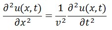
In geophysics we always encounter with the waves such as earthquake waves, sound waves, oscilating electric and magnetic field in electromagnetic radiation. Thus we need to understand the nature of the this physical phenomena. "Wave equation" can be derived basic equation of motion and restoring forces of differential equation. This equation describes the waves in time and space. Let's consider an ocean wave and assume that the displacement given by u(x,t), then the wave equation can be written as;
 The factor of the V is speed of the wave. Solution of this linear partial differential equation is;
 A: amplitude
k: constant
w: circular frequency
'phi'(greek letter): phase
Now if we fixed the boundary conditions there is no displacement at the end points;
function vs1d(xmin,xmax,n,w,phase)
%%%%%%%%%%%%%%%%%%%%
% Author: Mustafa DENIZ %
% Contact: mustafdeniz@itu.edu.tr %
%%%%%%%%%%%%%%%%%%%%%
tmax=2*pi/w; %maximum time
dt=0.05; %timestep
frms=round(tmax/dt); %number of frame
x=xmin:0.01:1; %grid x
for ii=1:frms-1;
plot(x,unodes(x,ii*dt,n,w,phase));
axis([xmin xmax -1.5 1.5])
m(ii)=getframe;
end
movie(m,3)
Subsequently we can change the nodes,phase length of string arbitrarily by typing this command, for example;
>>vs1d(0,1,1,1,2)
if we want see the third node just change value of n variable in command;
>>vs1d(0,1,3,1,2)
REFERENCES:
 The factor of the V is speed of the wave. Solution of this linear partial differential equation is;
 A: amplitude
k: constant
w: circular frequency
'phi'(greek letter): phase
Now if we fixed the boundary conditions there is no displacement at the end points;
u(0,t)=u(L,t)=0
Finally we have the standing wave that has nodes at the location of two endpoints. New solution for this specific problem is;
 Implementation this problem to matlab takes two steps, first create a function which calculates nodes, secondly create another function for plotting purpose;
function u=unodes(x,dt,n,w,phase)
u=cos(n*w*dt+phase).*sin(n*pi*x);
end
plotting function is;Finally we have the standing wave that has nodes at the location of two endpoints. New solution for this specific problem is;
 Implementation this problem to matlab takes two steps, first create a function which calculates nodes, secondly create another function for plotting purpose;
function u=unodes(x,dt,n,w,phase)
u=cos(n*w*dt+phase).*sin(n*pi*x);
end
function vs1d(xmin,xmax,n,w,phase)
%%%%%%%%%%%%%%%%%%%%
% Author: Mustafa DENIZ %
% Contact: mustafdeniz@itu.edu.tr %
%%%%%%%%%%%%%%%%%%%%%
tmax=2*pi/w; %maximum time
dt=0.05; %timestep
frms=round(tmax/dt); %number of frame
x=xmin:0.01:1; %grid x
for ii=1:frms-1;
plot(x,unodes(x,ii*dt,n,w,phase));
axis([xmin xmax -1.5 1.5])
m(ii)=getframe;
end
movie(m,3)
Subsequently we can change the nodes,phase length of string arbitrarily by typing this command, for example;
>>vs1d(0,1,1,1,2)
if we want see the third node just change value of n variable in command;
>>vs1d(0,1,3,1,2)
REFERENCES:
22 Haziran 2011 Çarşamba
Nonlinear Fitting Marquardt - Levenberg Algorithm
In this session I will study polynomial nonlinear fit Marquardt - Levenberg algorithm. The goal is how we can implement the methods to matlab.
First we consider our mathematical model fourth order polynomial;

Let's create the data and add gaussian distrubuted noise to our data, in matlab we just type these commands;
>> x=linspace(0,4,40); % create 40 datapoints between 0 and 4
>> a=-1; b=2; c=-3; d=-1; e=-30; % fit parameters
>> y=a.*x.^4+b.*x.^3+c.*x.^2+d.*x+e;
Now we've created the data. Matlab has a command as "randn" which generates normally distrubuted random numbers:
>> y=y+0.5*sqrt((max(abs(y)))).*randn(1,length(y)); %adds noise

Since our model is linear, it means there is no linear dependency among the parameters, we can expect that the solution would be unique. Marquardt-Levenberg solution of the equation;

A is the jacobian matrix which includes partial derivatives for each fit parameters, dx correction values and dy is the difference between theoretical and the observed data. Lambda is known as damping parameter.
Iterative solution has offered for nonlinear fit so our program will have a cycle which controls the number of iterations. Eeach iteration we will get the parameter correction values and add these values to our guess. Let's see the main structure of the code:
%%%%%%%%%%%%%%%%%%%%
% Author: Mustafa DENIZ %
% Contact: mustafdeniz@itu.edu.tr %
%%%%%%%%%%%%%%%%%%%%%
a=1; b=1; c=1; d=1,e=1; theta=5; %initial guesses
a0=a; b0=b; c0=c; d0=d; e0=e;
itnu=input('iteration number:');
for ii=1:itnu;
y=a.*x.^4+b.*x.^3+c.*x.^2+d.*x+e; %mathematical model
da=x.^4; db=x.^3; dc=x.^2; dd=x; de=ones(1,N) % partial derivatives
U=[da',db',dc',dd',de']; %Jacobian matrix
dy=yo-y; %obeserved-calculated
dp=(U'*U+theta*eye(5))\U'*dy'; %solving the system
a=a+dp(1); b=b+dp(2); c=c+dp(3); d=d+dp(4); e=e+dp(5); %add dp's to parameters
ai(ii)=a; bi(ii)=b; ci(ii)=c; di(ii)=d; ei(ii)=e;
gof(ii)=0.2*sum(sqrt(dy.^2)); %goodness of fit
figure(1)
plot(x,yo,'*')
title('calculated vs observed')
xlabel('x')
ylabel('amplitude')
hold on
plot(x,y,'r')
legend('observed','calculated')
end
%plot Goodness of fit
figure(2)
plot(gof,'-rs','LineWidth',2,'MarkerEdgeColor','g','MarkerFaceColor','b','MarkerSize',5)
xlabel('iteration number')
ylabel('Goodnes of fit')
%plot the parameters by iteration
figure(3)
subplot(3,2,1)
plot(0:itnu,[a0 ai],'-rs','LineWidth',2,'MarkerEdgeColor','g','MarkerFaceColor','b','MarkerSize',5)
title('Changing of a')
xlabel('iteration number')
ylabel('a')
subplot(3,2,2)
plot(0:itnu,[b0 bi],'-rs','LineWidth',2,'MarkerEdgeColor','g','MarkerFaceColor','b','MarkerSize',5)
title('Changing of b')
xlabel('iteration number')
ylabel('b')
subplot(3,2,3)
plot(0:itnu,[c0 ci],'-rs','LineWidth',2,'MarkerEdgeColor','g','MarkerFaceColor','b','MarkerSize',5)
title('Changing of c')
xlabel('iteration number')
ylabel('c')
subplot(3,2,4)
plot(0:itnu,[d0 di],'-rs','LineWidth',2,'MarkerEdgeColor','g','MarkerFaceColor','b','MarkerSize',5)
title('Changing of d')
xlabel('iteration number')
ylabel('d')
subplot(3,2,5)
plot(0:itnu,[e0 ei],'-rs','LineWidth',2,'MarkerEdgeColor','g','MarkerFaceColor','b','MarkerSize',5)
title('Changing of e')
xlabel('iteration number')
ylabel('e')
Even I've started with awful initial guesses solution has came up quickly because of the model parameters are linearly independent.

In an addition I did not weight the data nor the parameters. I assumed that the data is perfect and there is no uncertainty but for real life we know that those things should be there. Next time I will study fitting with SVD and add weighting the both parameters and the data.
20 Haziran 2011 Pazartesi
LU Decomposition
ONE SQUARE MATRIX = TWO TRIANGULAR MATRIX
A=LU
The factors are L and U triangular matrices. U is the upper triangular matrix with the pivots on diagonal. Eliminitaion takes A to U, reversing this step back U to A takes, L. L is lower triangular matrix and has all 1's its diagonal. Let's factorize a random matrix without row exchanges;
>>A=round(10*rand(n,n)) % creates n by n matrix (n=arbitrary)
%%%%%%%%%%%%%%%%%%%%
% Author: Mustafa DENIZ %
% Contact: mustafdeniz@itu.edu.tr %
%%%%%%%%%%%%%%%%%%%%%
[n,n]=size(A);
tolerance=1.e-8;
for k = 1:n
if abs(A(k, k)) < tolerance
end
L(k, k) = 1;
for i = k+1:n
L(i,k) = A(i, k) / A(k, k); %Multipliers for column k are put into L
for j = k+1:n %Elimination beyond row k and column k.
A(i, j) = A(i, j) - L(i, k)*A(k, j);
end
end
for j = k:n
U(k, j) = A(k, j);
end
end
Matlab has a command also for LU factorization;
>> [U,L]=lu(A)
References:
Strang. G., 2009. Introduction to Linear Algebra, Fourth Edition, Wellesley Cambridge Press.
William H.P. et al, 2007. Numerical Recipes 3rd Edition: The Art of Scientific Computing, Cambridge University Press.
Kaydol:
Yorumlar (Atom)